 |
Slow feature analysis yields a rich repertoire of complex-cell properties - Additional Material |
This page contains additional material to the papers
Berkes, P. and Wiskott, L. (2005).
Slow feature analysis yields a rich repertoire of complex cell properties.
Journal of Vision, 5(6), 579-602,
http://journalofvision.org/5/6/9/,
doi:10.1167/5.6.9.
(bibtex,
abstract,
paper)
and
Berkes, P. and Wiskott, L. (2003).
Slow feature analysis yields a rich repertoire of complex-cell properties.
Cognitive Sciences EPrint Archive (CogPrint) 2804,
http://cogprints.ecs.soton.ac.uk/archive/00002804/
(bibtex,
abstract,
.ps,.pdf)
Table of contents
- Abstract
- Analysis pages of some units
- Overview of the optimal excitatory stimuli
- Overview of the circular response images
(Units #1-9, Units #10-18, Units #19-27, Units #28-30) - Overview of the hexagonal response images
(Units #1-9, Units #10-18, Units #19-27, Units #28-30) - Population statistics
- Relative contribution of the quadratic, linear and constant terms
- Optimal excitatory stimuli of the control experiments
- Matlab program to perform simulations with the temporal slowness model of self-organization of complex-cell receptive fields.
Related pages
- Index page ot the research project "Slowness as a computational principle for the visual cortex"
- Slow Feature Analysis: Unsupervised Learning of Invariances (by Laurenz Wiskott)
- Applying Slow Feature Analysis to Image Sequences Yields a Rich Repertoire of Complex Cell Properties - Additional Material
For further information please refer to the cited papers or mail to

Abstract
In this study, we investigate temporal slowness as a learning principle for receptive fields using slow feature analysis, a new algorithm to determine functions that extract slowly varying signals from the input data. We find that the learned functions trained on image sequences develop many properties found also experimentally in complex cells of primary visual cortex, such as direction selectivity, non-orthogonal inhibition, end-inhibition and side-inhibition. Our results demonstrate that a single unsupervised learning principle can account for such a rich repertoire of receptive field properties.
Analysis pages of some units
The analysis pages are automatically generated at the end of a simulation and contain several informations about the learned units.Description of an analysis page
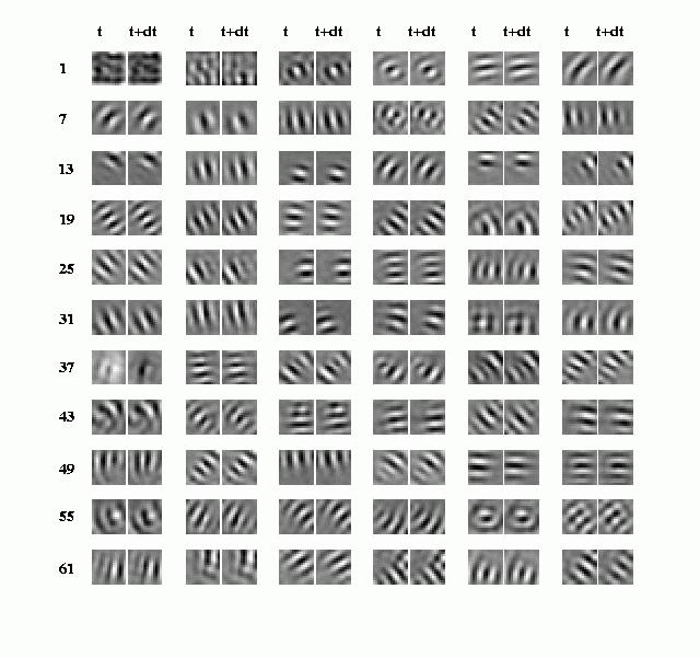
Overview of the optimal excitatory stimuli
|
| Figure 1, Overview of the optimal excitatory stimuli. The above image gives an overview of the optimal excitatory stimuli (S+) for the first (the slowest) 66 units resulting from the simulation described in the paper. For each S+, the left patch shows the stimulus at time t, and the right one the stimulus at time t+dt. A difference in the two patches thus hints at the time behavior of a unit. Most S+ look like Gabor wavelets (in agreement with physiological data), i.e. the units respond best to oriented edges. All the units shown in the image but the first two have been classified as complex cells from their response characteristics. |
Overview of the circular response images
Description of the response images
| Units #1-9 | Units #10-18 | Units #19-27 | Units #28-30 |
Overview of the hexagonal response images
Description of the response images
| Units #1-9 | Units #10-18 | Units #19-27 | Units #28-30 |
Population statistics
a) |
b) |
|
c) |
||
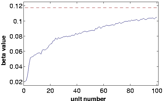
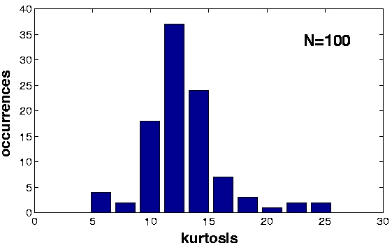
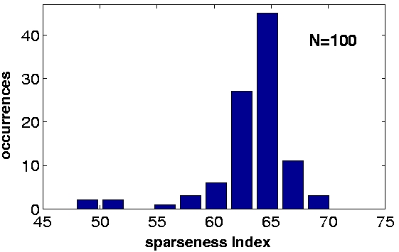
| Figure 2, Output statistics. We collected the responses of the units to ca. 400,000 previously unseen frames and computed some statistics: a) The beta values of the first 100 units in the simulation. The red dashed line is the beta value of the visual input sequences. The units maintain a slowly varying output also with respect to novel data. Also their order remain fixed up to some fluctuations. b) The kurtosis of the first 100 units in the simulation. c) The sparseness index of the first 100 units in the simulation. (Click on the images to enlarge them.) | ||
Relative contribution of the quadratic, linear and constant terms
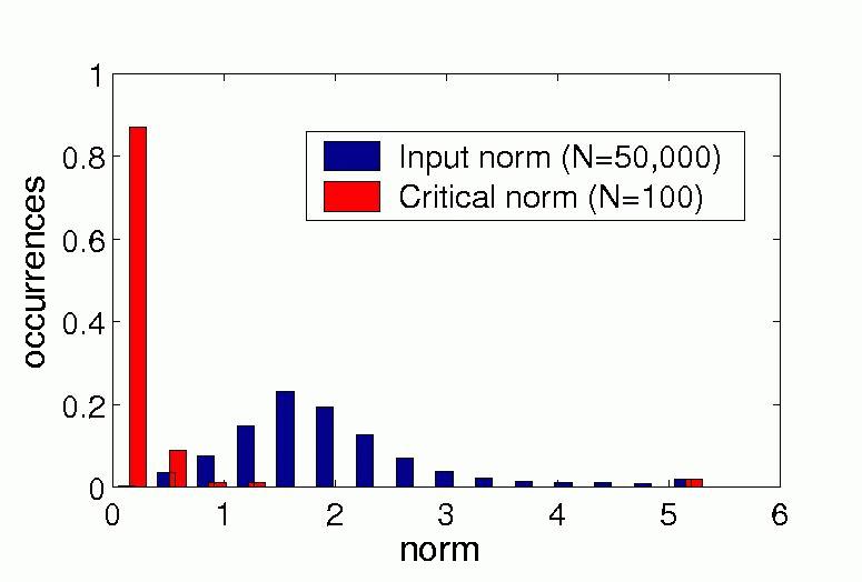
Our units are polynoms of degree 2 in the visual input, and are composed of a quadratic term (monoms of degree 2), a linear term (monoms of degree 1) and a constant term. We are interested in their relative contribution to the output. Intuitively, the linear term would dominate for input vectors with a small norm, while the quadratic term would dominate for large input vectors. We characterize the relative contribution of the quadratic and of the linear term by the critical norm, i.e. the norm at which the quadratic term first dominates. The critical norm is thus the norm lambda that satisfies the following equation:

where q(x) and l(x) are the quadratic and the linear term of the polynom, respectively. Under the critical norm the linear term dominates while above it the quadratic term dominates. Figure 3a) shows the distribution of the critical norm and the distribution of the norm of the input vectors in our simulation. The critical norms are usually small in comparison to the typical input, which means that the quadratic term dominates in the typical regime.
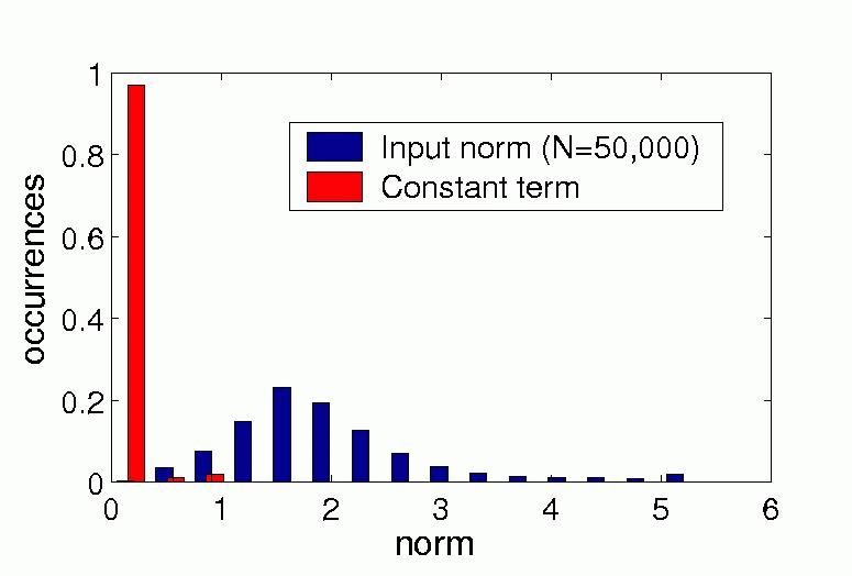
Figure 3b) shows the distribution of the absolute value of the constant term and the distribution of the norm of the input vectors in our simulation. The constant term is very small in almost all units and thus gives only a small contribution to the output.
Optimal excitatory stimuli of the control experiments
| Control Experiment 1 | Control Experiment 2 |
